0CCh Blog

机器学习练习题1

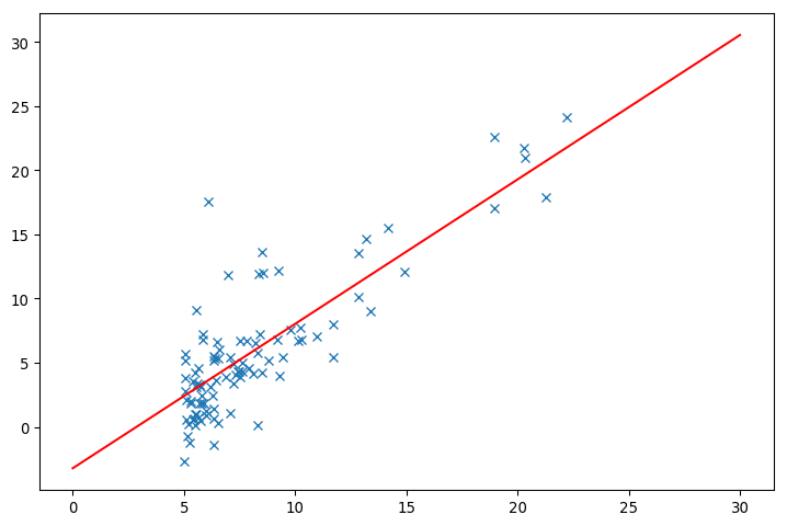
掐指一算,已经有三个月没有更新blog了。因为最近一直在学习机器学习的内容,所以没空也没有新鲜的技术值得写下来分享。还好经过一段时间的积累(学习线性代数和概率论),机器学习这块内容也算是入门了。这是机器学习的第一个习题,线性回归。用最直白的话来说,就是用函数去拟合数据分布,从而达到预测新数据的效果。需要的知识是矩阵的计算,最小二乘法以及求偏微分。

关键的公式只有两个:

那么最后需要确定的只剩下一个,我们希望用什么样的曲线去拟合样本,这个就需要经验和尝试了。这里的练习只需要用直线来拟合就足够了: \( h_\theta(x) = \theta^{T}x = \theta_{0}+\theta_{1}x_{1} \) .

# -*- coding: utf-8 -*-

import numpy as np
import matplotlib.pyplot as plt

data = np.loadtxt('ex1data1.txt', delimiter=',');

# 分离样本数据输入X和输出Y
X = np.concatenate((np.ones((len(data),1)), data[:,0].reshape((len(data),1))), axis=1)
theta = np.random.randn(2,1)
Y = data[:,1].reshape((len(data),1))

# 为了加速计算,把除法优化位乘法
alpha = 0.01
div_m = 1 / len(data);

for loop_count in range(1000):
Y1 = X.dot(theta)
# 根据公式计算损失
cost = ((Y-Y1)**2).sum() * 0.5 * div_m;
print(cost)
# 更新参数
for i in range(2):
theta[i, 0] = theta[i, 0] - alpha * div_m * (np.diagflat(X[:, i]) * (Y1 - Y)).sum()

# 最后把拟合直线画出来
Xl = np.linspace(0, 30, 100)
Yl = Xl * theta[1, 0] + theta[0, 0]

plt.plot(data[:,0],data[:,1],'x', Xl, Yl, 'r')

2018-06-23-machine-learning-ex1